![]()
Since its resurgence in the 90s Multi-agent models have been a close companion of evolutionary linguistics (which for me subsumes both the study of the evolution of Language with a capital L as well as language evolution, i.e. evolutionary approaches to language change). I’d probably go as far as saying that the early models, oozing with exciting emergent phenomena, actually helped in sparking this increased interest in the first place! But since multi-agent modelling is more of a ‘tool’ rather than a self-contained discipline, there don’t seem to be any guides on what makes a model ‘good’ or ‘bad’. Even more importantly, models are hardly ever reviewed or discussed on their own merits, but only in the context of specific papers and the specific claims that they are supposed to support.
This lack of discussion about models per se can make it difficult for non-specialist readers to evaluate whether a certain type of model is actually suitable to address the questions at hand, and whether the interpretation of the model’s results actually warrants the conclusions of the paper. At its worst this can render the modelling literature inaccessible to the non-modeller, which is clearly not the point. So I thought I’d share my 2 cents on the topic by scrutinising a few modelling papers and highlight some caveats, and hopefully also to serve as a guide to the aspiring modeller!
Anybody who’s ever gotten her hands dirty playing around with a multi-agent simulation will know how awesome it feels to send a program off for execution and wait a few seconds for it to produce a mountain of data that would have taken weeks or months to collect through classic psychological experimenting. This is the awesomeness of computational modelling, but it is also a curse. Because however tempting it is to run 1.000 instances of a stochastic simulation for 100.000 iterations each in 3.072 different conditions, all that data that is so easily produced will not only clog up your hard disk space, but it will also still need analysing.
The source of this luxury problem is that, rather than meticulously setting up two or maybe four conditions in which a human subject, acting as a blackbox, will hopefully perform in significantly different ways, it is very tempting (and admittedly very interesting!) for modellers to think about all the possible factors that might or might not lead to different behaviours, and implement them. More interestingly, because the unknown variable in multi-agent simulations are the interactions and cumulative effects we are free to not only vary environmental variables like population size and interaction patterns, but also control every little aspect of the agents’ individual behaviour. This means that in comparison to psychological experiments computational models will typically have many more parameters, many of which are continuous, leading to more and also more complex interactions between all of those parameters.
So no matter how ‘complete’ or ‘realistic’ you would like to make your model, any nonessential parameter n+1 that you put in will strike back in the form of a multiplicity of the amount of data and n (potentially nonlinear) interactions with all the other parameters which will be a pain to analyse, to fit, let alone to understand.
The first and most obvious point is of course that you ought to study (or in the case of modelling, make up) “the simplest system you think has the properties you are interested in” (Platt 1964), i.e. keep the number of parameters low! Having fewer parameters does not only allow you to sample the parameter space more exhaustively, it also makes eyeballing the data for interactions a lot easier, which can be followed up by some informed fitting of a descriptive model to the data.
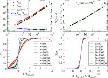
A great (but rare) example that I found on Toolerant of such an approach is the rigorous analysis of the Minimal strategy in the Naming Game by (Baronchelli et al. 2006). Their data is abundant, their model fits quantified, their figures mesmerising – and all that to study the impact of a single parameter (population size). I am not aware of any equally exhaustive and convincing studies of similarly interesting models investigating more than one parameter, most likely because precisely quantifying their interactions becomes complicated very quickly.
What I’m talking about here in terms of tractability are the natural limitations of what is called numerical modelling. Numerical modelling means that we determine the state that a model is in by using an incremental time-stepping procedure, which we have to iterate to learn about the development of the model over time. The results we get from such models are (as the name suggests) purely numerical, so if you want to study the model’s behaviour using different initial conditions you have to feed in different numbers at the start and run the same time-stepping procedure all over again. What’s worse, our updating function will usually contain some nondeterministic component, e.g. to randomise the order in which agents interact, which means that we will have to run the same condition multiple times to determine the interaction between the randomness and the model’s behaviour. The only exception to this general rule is when there is a transparent relationship between the probability distribution of the random variable and our updating function. In such cases we can sometimes run a numerical simulation of the development of the probability distribution over model states instead of running individual instances of our model, but this will generally not be the case. In most cases there will be nontrivial interactions where small quantitative differences in the random variables will lead to qualitatively different model behaviour, so we have to resort to running a large number of iterations using the same initial conditions just to get an idea of how our random influences affect the model.
That’s what makes numerical models a bit of a pain. They are (too) easy to run and you can implement almost anything you like with them, but they can be an absolute pain to analyse and, more problematically, it’s very difficult to draw any strict conclusions from them. This is probably also the reason why, following a frantic period of computational modelling from the mid-90s to the mid-00s, there have been significantly less simulations of evolutionary linguistics stuff carried out (or at least published) since then. Following the initial excitement over the very first results came a bit of a modelling hangover, most likely caused by some sort of resignation over just what we’re supposed to make of their results (de Boer 2012).
There is an alternative to numerical models though, and one that I would say is preferrable wherever possible, namely analytical modelling. Analytical just means that whatever model we happen to have cooked up, complete with parameter-controlled individual behaviour, parameter-controlled interactions and possibly some random components as well, has a mathematical closed form solution. “What on earth does that even mean?” I hear you asking. That just means that there is a solution to the equations which describe the changes to the state of our model (the time-stepping or update function that is called on every iteration in a numerical model) that can be expressed as an analytic function. If we were to squeeze our numerical model into an equation, it would most likely look something like xt = fα,λ,θ,...(xt-1), where xt captures the state of the model (i.e. the current prevalence of different traits/the agents and the languages they currently speak…) at time t and f applies the changes with which we update our population at every time step, the details of which are controlled by the parameters α, λ, θ etc. The observant reader will have noticed that this equation contains a recursion to xt-1, so if we want to know the state of our model after t iterations we have to first compute the state after t-1 iterations all the way down to 0, where we can just refer to the initial state x0 which is given. Evaluating this formula for a specific combination of parameters is basically what we do when we run a computer simulation.
Now the art of mathematical modelling is to transform this equation into something that looks like x(t) = f(x0, t, α, λ, θ,...) where f has to be a function of the given parameters containing only simple mathematical operations like addition, multiplication, the odd exponential or trigonometric function, but crucially no recursion to f(). If we find such an f then this is the analytical solution to our model, and if we want to know the state of our model after a certain number of iterations (note how t has become a simple parameter of f) given certain parameters and initial conditions we just have to fill in those values and perform a straightforward evaluation of this simple formula.
What’s more, because our parameters are explicit in f(), we might even be able to read off their individual effects on the overall dynamics without having to try out specific values. With a bit of luck we will be able to tell which parameters shift our system state x in which direction, whether their influence on the model is linear, quadratic, exponential, just constant, or whether they don’t affect the dynamics at all. (This might seem bizarre but I know of at least two papers covering computer simulations which discuss aspects of the model that are in fact completely irrelevant for the overall dynamics. One of them contains a parameter setting which completely cuts off the influences from another part of the model, but the results are still discussed as if the influence was there. The other contains a description of an aspect of the model that important influence is ascribed to, but the condition that would cause this part of the model to become active are never fulfilled, i.e. it describes bits of the simulation code that can in fact never be reached. In both cases it doesn’t seem like the authors have realised this. Spelling a model out in mathematical equations might not always be possible but it is certainly worthwhile to try and transcend purely verbal description to make it clearer what is actually going on.) Where was I? Oh yes, analytical models might even allow you to see whether the influence of specific parameters increases or decreases over time, whether the model converges towards some increasingly stable end state or whether it keeps on fluctuating, possibly exhibiting periodic behaviour etc etc.
It is important to note that analytical and numerical modelling are not two incompatible things. The ‘model’ itself, i.e. a description of how a system of certain shape changes over time, precedes both, analytical and numerical modelling are merely two different ways to figure out what the predictions of that model are. It is true however that some decisions in drawing up the model are taken with a particular kind of modelling approach in mind. Some of the core components of any model are going to be motivated or justified by common sense (an agent encountering a new convention should presumably add this form to his memory rather than, say, ignore the form but nevertheless scramble or invert the scores of all the conventions he already has in his memory), but other decisions are pretty arbitrary (de Boer 2012), in particular when it comes to how exactly continuous values/variables are updated. So while in numerical simulations you will tend to go for operations which are computationally cheap (examples being any multi-agent simulations of conventionalisation where scores of competing variants are simply incremented or decremented, still the cheapest operations on modern computers), analytic models are likely to make use of functions which might be computationally unwieldy, but mathematically very well understood (examples for this would be the use of an exponential distance function in (Nowak et al. 1999, p.2132), or the definition of the sample prediction function in Reali & Griffiths 2010, p.431-432).
It is natural to be a bit puzzled or sceptical when you come across those arbitrary choices made in papers – would the model behave completely different if they’d chosen a slightly different function? But one has to concede that in coming up with a model, some arbitrary choices have to be taken anyway. And if that’s the case then they might as well be taken in a way that simplifies whatever you’re doing, whether it’s numerical computation or mathematical analysis – because without that guided choice we might not have any results at all.
So while a lot of models can be implemented both numerically and analytically (which is a great way to cross-check their results!), some are only amenable to either approach. For many complex models analytical solutions are not obtainable, but conversely some analytical results based on infinite population sizes or continuous time models (where the updates between model states become infinitesimally small) can simply not be captured by running a discrete time-stepping function. But such models are the exception, and in most cases what will happen is that you implement and tinker with a numerical model first and, stumbling upon interesting results, attempt to figure out whether the behaviour can be captured and predicted analytically which would, if you’re lucky, relieve you from having to exhaustively run those 3.071 other conditions as well.
A brilliant example of how numerical and analytical models often coincide can be found in Jäger 2008 (link below) in which he shows that the behaviour of two seemingly disparate numerical models of language evolution (one an exemplar theory model of the evolution of phoneme categories a la Wedel/Pierrehumbert, the other (Nowak et al. 2001)’s evolutionary model of iterated grammar acquisition) can in fact both be captured by the Price equation, which is a general solution to predict the development of any system undergoing change by replication (i.e. evolution). The paper is a great read and easily understandable for anyone who’s not afraid of a bit of stats, so I highly recommend having a look at it!
To summarise, having an analytical model simply adds concision and predictive power to your results. But if analytical modelling is oh so awesome, why isn’t everyone doing it then? The first part of the problem is that a lot of models, and certainly a lot of the more interesting and realistic ones, simply don’t have such a closed-form solution. The ones that are solvable lead to powerful and irrevocable results though and it is very instructive to try and reconstruct them yourself, something that most biologists and the odd economist but sadly not enough social scientists will have some experience with.
A second problem is that even if an analytic solution is in principle obtainable, it is still far from trivial to do so, and pretty futile to attempt unless you have a background in maths or physics (disclaimer: I have neither and I have so far also not produced any analytical models myself).
The crux is that while not a lot of models are exactly solvable, many of them can be approximated by making certain assumptions, which is where we can finally look at the tradeoff between numerical and analytical models! In the aforementioned case where there is some stochastic component in the system (i.e. some aspect of the system is specified by a probability distribution rather than a value), any analytical solution would have to be a function transforming this distribution into a another distribution, which can get hairy very very quickly. So while it will typically not be possible to obtain a description of the entire distribution over model states, we can try to get at a description of the average state that the model will be in. This is often done based on so-called mean field assumptions, i.e. by disregarding the fluctuations around this average caused by stochastic interferences and sampling effects.
Most analytical models you encounter in the literature will rely on such approximations, and it is important to realise that they influence how we may interpret their results. This is something that can easily get lost in the quick succession of mathematical transformations and unwieldy equations full of greek characters. Most readers without a background in maths have no choice but to either disregard such models because they cannot evaluate their validity themselves, or otherwise accept their conclusions at face value. Both of these options are far from ideal of course and, given the merits of analytic models that I outlined above, it is absolutely worthwhile to consider those models and try to understand what their approximations mean for the results.
Funnily enough all this was just intended to be the introduction to a post in which I wanted to have a closer look at two analytical modelling papers and their conclusions, but since it might have some value by itself I think I’m gonna leave it at this for now! So check back in a week or so for some applied model dissection!
References
Baronchelli, Andrea, Felici, Maddalena, Loreto, Vittorio, Caglioti, Emanuele, & Steels, Luc (2006). Sharp transition towards shared vocabularies in multi-agent systems Journal of Statistical Mechanics: Theory and Experiment, 2006 (06) DOI: 10.1088/1742-5468/2006/06/P06014
de Boer, Bart (2012). Modelling and Language Evolution: Beyond Fact-Free Science Five Approaches to Language Evolution: Proceedings of the Workshops of the 9th International Conference on the Evolution of Language, 83-92
Jäger, Gerhard (2008). Language evolution and George Price’s “General Theory of Selection” Language in flux: dialogue coordination, language variation, change and evolution, Communication, mind & language 1, 53-80 Other: http://www.sfs.uni-tuebingen.de/~gjaeger/publications/leverhulme.pdf
Platt, John R (1964). Strong inference Science, 146 (3642), 347-353 : 10.1126/science.146.3642.347
Nowak Martin A, Krakauer David C, & Dress Andreas (1999). An error limit for the evolution of language Proceedings of the Royal Society B: Biological Sciences, 266 (1433), 2131-2136 PMID: 10902547
Nowak, Martin A, Komarova, Natalia L, & Niyogi, Partha (2001). Evolution of universal grammar Science, 291 (5501), 114-118 PMID: 11141560
Reali, Florencia, & Griffiths, Thomas L (2009). Words as alleles: connecting language evolution with Bayesian learners to models of genetic drift Proceedings of the Royal Society B: Biological Sciences, 277 (1680), 429-436 DOI: 10.1098/rspb.2009.1513
Awesome post! You have just handily explained to me why I got a job with physicists.
de Boer 2012’s not in the reference list!
Woop thanks for that, fixed now!